Data transformation
介绍
可视化是生成洞察力的重要工具,但很少有情况下你会得到完全符合你所需的图形的数据形式。通常情况下,你需要创建一些新的变量或摘要来回答你的数据问题,或者你可能只想重命名变量或重新排序观察结果,以使数据更容易处理。在本章中,你将学习如何做到这一点(以及更多!),这将通过使用 dplyr 包和一个新的数据集介绍数据转换,该数据集包含了 2013 年从纽约市起飞的航班信息。
本章的目标是为你概述转换数据框的所有关键工具。我们将从操作数据框的行和列的函数开始,然后回过头来更多地讨论管道,这是一个将动词组合在一起的重要工具。然后我们将介绍使用分组的能力。我们将在章节结束时通过一个案例研究来展示这些功能,并在后续章节中更详细地讨论这些功能,因为我们开始深入研究特定类型的数据(例如数字、字符串、日期)。
先决条件
在本章中,我们将重点介绍 dplyr 包,这是 tidyverse 的另一个核心成员。我们将使用 nycflights13 包中的数据来说明关键思想,并使用 ggplot2 来帮助我们理解数据。
library(nycflights13)
library(tidyverse)
#> ── Attaching core tidyverse packages ───────────────────── tidyverse 2.0.0 ──
#> ✔ dplyr     1.1.4     ✔ readr     2.1.5
#> ✔ forcats   1.0.0     ✔ stringr   1.5.1
#> ✔ ggplot2   3.5.1     ✔ tibble    3.2.1
#> ✔ lubridate 1.9.3     ✔ tidyr     1.3.1
#> ✔ purrr     1.0.2
#> ── Conflicts ─────────────────────────────────────── tidyverse_conflicts() ──
#> ✖ dplyr::filter() masks stats::filter()
#> ✖ dplyr::lag()    masks stats::lag()
#> ℹ Use the conflicted package (<http://conflicted.r-lib.org/>) to force all conflicts to become errors
请仔细注意加载 tidyverse 时打印的冲突消息。它告诉你 dplyr 覆盖了基础 R 中的一些函数。如果你想在加载 dplyr 后使用这些函数的基础版本,你需要使用它们的完整名称:stats::filter() 和 stats::lag()。到目前为止,我们大多忽略了函数来自哪个包,因为大多数情况下这并不重要。然而,知道函数来自哪个包可以帮助你找到帮助和相关函数,所以当我们需要准确指定函数来自哪个包时,我们将使用与 R 相同的语法:packagename::functionname()。
nycflights13
为了探索基本的 dplyr 动词,我们将使用 nycflights13::flights。这个数据集包含了 2013 年从纽约市出发的所有 336,776 趟航班。数据来自美国运输统计局,并在 ?flights 中有文档记录。
flights
#> # A tibble: 336,776 × 19
#>    year month   day dep_time sched_dep_time dep_delay arr_time sched_arr_time
#>   <int> <int> <int>    <int>          <int>     <dbl>    <int>          <int>
#> 1  2013     1     1      517            515         2      830            819
#> 2  2013     1     1      533            529         4      850            830
#> 3  2013     1     1      542            540         2      923            850
#> 4  2013     1     1      544            545        -1     1004           1022
#> 5  2013     1     1      554            600        -6      812            837
#> 6  2013     1     1      554            558        -4      740            728
#> # ℹ 336,770 more rows
#> # ℹ 11 more variables: arr_delay <dbl>, carrier <chr>, flight <int>, …
flights 是一个 tibble,是 tidyverse 中使用的一种特殊类型的数据框,用于避免一些常见的陷阱。tibble 和数据框之间最重要的区别在于它们的打印方式;它们设计用于大型数据集,因此它们只显示前几行和一屏幕上适合的列。有几种方法可以查看全部内容。如果你正在使用 RStudio,最方便的方法可能是使用 View(flights),它将打开一个交互式的可滚动和可过滤的视图。否则,你可以使用 print(flights, width = Inf) 来显示所有列,或者使用 glimpse():
glimpse(flights)
#> Rows: 336,776
#> Columns: 19
#> $ year           <int> 2013, 2013, 2013, 2013, 2013, 2013, 2013, 2013, 2013…
#> $ month          <int> 1, 1, 1, 1, 1, 1, 1, 1, 1, 1, 1, 1, 1, 1, 1, 1, 1, 1…
#> $ day            <int> 1, 1, 1, 1, 1, 1, 1, 1, 1, 1, 1, 1, 1, 1, 1, 1, 1, 1…
#> $ dep_time       <int> 517, 533, 542, 544, 554, 554, 555, 557, 557, 558, 55…
#> $ sched_dep_time <int> 515, 529, 540, 545, 600, 558, 600, 600, 600, 600, 60…
#> $ dep_delay      <dbl> 2, 4, 2, -1, -6, -4, -5, -3, -3, -2, -2, -2, -2, -2,…
#> $ arr_time       <int> 830, 850, 923, 1004, 812, 740, 913, 709, 838, 753, 8…
#> $ sched_arr_time <int> 819, 830, 850, 1022, 837, 728, 854, 723, 846, 745, 8…
#> $ arr_delay      <dbl> 11, 20, 33, -18, -25, 12, 19, -14, -8, 8, -2, -3, 7,…
#> $ carrier        <chr> "UA", "UA", "AA", "B6", "DL", "UA", "B6", "EV", "B6"…
#> $ flight         <int> 1545, 1714, 1141, 725, 461, 1696, 507, 5708, 79, 301…
#> $ tailnum        <chr> "N14228", "N24211", "N619AA", "N804JB", "N668DN", "N…
#> $ origin         <chr> "EWR", "LGA", "JFK", "JFK", "LGA", "EWR", "EWR", "LG…
#> $ dest           <chr> "IAH", "IAH", "MIA", "BQN", "ATL", "ORD", "FLL", "IA…
#> $ air_time       <dbl> 227, 227, 160, 183, 116, 150, 158, 53, 140, 138, 149…
#> $ distance       <dbl> 1400, 1416, 1089, 1576, 762, 719, 1065, 229, 944, 73…
#> $ hour           <dbl> 5, 5, 5, 5, 6, 5, 6, 6, 6, 6, 6, 6, 6, 6, 6, 5, 6, 6…
#> $ minute         <dbl> 15, 29, 40, 45, 0, 58, 0, 0, 0, 0, 0, 0, 0, 0, 0, 59…
#> $ time_hour      <dttm> 2013-01-01 05:00:00, 2013-01-01 05:00:00, 2013-01-0…
在这两个视图中,变量名称后面跟着缩写,告诉你每个变量的类型:
dplyr基础
你即将学习到主要的 dplyr 动词(函数),这将使你能够解决绝大多数数据处理挑战。但在讨论它们的个别差异之前,值得指出它们共同的特点:
- 第一个参数始终是数据框。
- 后续的参数通常描述要操作的列,使用变量名称(不使用引号)。
- 输出始终是一个新的数据框。
因为每个动词都可以很好地执行一件事情,所以解决复杂的问题通常需要组合多个动词,我们将使用管道,|>。我们将在第 3.4 节中更详细地讨论管道,但简单来说,管道将其左侧的内容传递给其右侧的函数,因此 x |> f(y) 等同于 f(x, y),x |> f(y) |> g(z) 等同于 g(f(x, y), z)。读音最简单的方法是“then”。这使得即使你尚未学习细节,也可以理解以下代码的意义:
flights |>
  filter(dest == "IAH") |>
  group_by(year, month, day) |>
  summarize(
    arr_delay = mean(arr_delay, na.rm = TRUE)
  )
dplyr 的动词根据它们操作的内容分为四组:行、列、组或表。在接下来的章节中,你将学习到行、列和分组的最重要的动词,然后我们将在第 19 章中回顾作用于表的连接动词。让我们开始吧!
行
操作数据集行的最重要的动词是 filter() 和 arrange()。filter() 根据列的值保留行,而 arrange() 则根据行的值对行进行排序。这两个函数只影响行,列保持不变。我们还会讨论 distinct(),它找到具有唯一值的行,但与 arrange() 和 filter() 不同,它还可以选择性地修改列。
filter()
filter() 允许你根据列的值保留行。第一个参数是数据框。第二个及后续的参数是必须为真以保留行的条件。例如,我们可以找到所有出发晚于 120 分钟(两小时)的航班:
flights |>
  filter(dep_delay > 120)
#> # A tibble: 9,723 × 19
#>    year month   day dep_time sched_dep_time dep_delay arr_time sched_arr_time
#>   <int> <int> <int>    <int>          <int>     <dbl>    <int>          <int>
#> 1  2013     1     1      848           1835       853     1001           1950
#> 2  2013     1     1      957            733       144     1056            853
#> 3  2013     1     1     1114            900       134     1447           1222
#> 4  2013     1     1     1540           1338       122     2020           1825
#> 5  2013     1     1     1815           1325       290     2120           1542
#> 6  2013     1     1     1842           1422       260     1958           1535
#> # ℹ 9,717 more rows
#> # ℹ 11 more variables: arr_delay <dbl>, carrier <chr>, flight <int>, …
除了 >(大于)外,你还可以使用 >=(大于或等于)、<(小于)、<=(小于或等于)、==(等于)和 !=(不等于)等条件。你还可以使用 & 或 , 来组合条件,表示“和”(检查两个条件),或使用 | 表示“或”(检查任一条件):
# Flights that departed on January 1
flights |>
  filter(month == 1 & day == 1)
#> # A tibble: 842 × 19
#>    year month   day dep_time sched_dep_time dep_delay arr_time sched_arr_time
#>   <int> <int> <int>    <int>          <int>     <dbl>    <int>          <int>
#> 1  2013     1     1      517            515         2      830            819
#> 2  2013     1     1      533            529         4      850            830
#> 3  2013     1     1      542            540         2      923            850
#> 4  2013     1     1      544            545        -1     1004           1022
#> 5  2013     1     1      554            600        -6      812            837
#> 6  2013     1     1      554            558        -4      740            728
#> # ℹ 836 more rows
#> # ℹ 11 more variables: arr_delay <dbl>, carrier <chr>, flight <int>, …

# Flights that departed in January or February
flights |>
  filter(month == 1 | month == 2)
#> # A tibble: 51,955 × 19
#>    year month   day dep_time sched_dep_time dep_delay arr_time sched_arr_time
#>   <int> <int> <int>    <int>          <int>     <dbl>    <int>          <int>
#> 1  2013     1     1      517            515         2      830            819
#> 2  2013     1     1      533            529         4      850            830
#> 3  2013     1     1      542            540         2      923            850
#> 4  2013     1     1      544            545        -1     1004           1022
#> 5  2013     1     1      554            600        -6      812            837
#> 6  2013     1     1      554            558        -4      740            728
#> # ℹ 51,949 more rows
#> # ℹ 11 more variables: arr_delay <dbl>, carrier <chr>, flight <int>, …
当你结合 | 和 == 时有一个有用的快捷方式:%in%。它会保留变量等于右侧值之一的行:
# A shorter way to select flights that departed in January or February
flights |>
  filter(month %in% c(1, 2))
#> # A tibble: 51,955 × 19
#>    year month   day dep_time sched_dep_time dep_delay arr_time sched_arr_time
#>   <int> <int> <int>    <int>          <int>     <dbl>    <int>          <int>
#> 1  2013     1     1      517            515         2      830            819
#> 2  2013     1     1      533            529         4      850            830
#> 3  2013     1     1      542            540         2      923            850
#> 4  2013     1     1      544            545        -1     1004           1022
#> 5  2013     1     1      554            600        -6      812            837
#> 6  2013     1     1      554            558        -4      740            728
#> # ℹ 51,949 more rows
#> # ℹ 11 more variables: arr_delay <dbl>, carrier <chr>, flight <int>, …
我们将在第 12 章中更详细地回顾这些比较和逻辑运算符。
当你运行 filter() 时,dplyr 执行过滤操作,创建一个新的数据框,然后将其打印出来。它不会修改现有的 flights 数据集,因为 dplyr 函数从不修改它们的输入。要保存结果,你需要使用赋值运算符 <-:
jan1 <- flights |>
  filter(month == 1 & day == 1)
常见错误
当你刚开始使用 R 时,最容易犯的错误是在测试相等性时使用 = 而不是 ==。filter() 会在发生这种情况时通知你:
flights |>
  filter(month = 1)
#> Error in `filter()`:
#> ! We detected a named input.
#> ℹ This usually means that you've used `=` instead of `==`.
#> ℹ Did you mean `month == 1`?
另一个错误是将“或”语句写成英语中的样子:
flights |>
  filter(month == 1 | 2)
在没有引发错误的意义上,这种方法“会奏效”,但不会和想象中的效一致,因为 | 首先检查 month == 1 条件,然后检查条件 2,这不是一个明智的条件。我们将在第 12.3.2 节中更详细地了解到这里发生了什么以及为什么。
arrange()
arrange() 根据列的值更改行的顺序。它接受一个数据框和一组列名(或更复杂的表达式)进行排序。如果你提供多个列名,每个额外的列将用于在前面列的值中打破关系。例如,以下代码按出发时间排序,出发时间分布在四列中。我们首先得到最早的年份,然后是每年最早的月份等。
flights |>
  arrange(year, month, day, dep_time)
#> # A tibble: 336,776 × 19
#>    year month   day dep_time sched_dep_time dep_delay arr_time sched_arr_time
#>   <int> <int> <int>    <int>          <int>     <dbl>    <int>          <int>
#> 1  2013     1     1      517            515         2      830            819
#> 2  2013     1     1      533            529         4      850            830
#> 3  2013     1     1      542            540         2      923            850
#> 4  2013     1     1      544            545        -1     1004           1022
#> 5  2013     1     1      554            600        -6      812            837
#> 6  2013     1     1      554            558        -4      740            728
#> # ℹ 336,770 more rows
#> # ℹ 11 more variables: arr_delay <dbl>, carrier <chr>, flight <int>, …
你可以在 arrange() 内部的列上使用 desc() 以按降序(从大到小)重新排序数据框。例如,此代码按航班延误时间从最长到最短排序:
flights |>
  arrange(desc(dep_delay))
#> # A tibble: 336,776 × 19
#>    year month   day dep_time sched_dep_time dep_delay arr_time sched_arr_time
#>   <int> <int> <int>    <int>          <int>     <dbl>    <int>          <int>
#> 1  2013     1     9      641            900      1301     1242           1530
#> 2  2013     6    15     1432           1935      1137     1607           2120
#> 3  2013     1    10     1121           1635      1126     1239           1810
#> 4  2013     9    20     1139           1845      1014     1457           2210
#> 5  2013     7    22      845           1600      1005     1044           1815
#> 6  2013     4    10     1100           1900       960     1342           2211
#> # ℹ 336,770 more rows
#> # ℹ 11 more variables: arr_delay <dbl>, carrier <chr>, flight <int>, …
请注意,行数并未改变 - 我们只是排列数据,而不是过滤它。
distinct()
distinct() 函数用于在数据集中找到所有唯一的行,因此从技术上讲,它主要作用于行。然而,大多数情况下,你可能希望得到某些变量的唯一组合,因此你也可以选择提供列名:
# Remove duplicate rows, if any
flights |>
  distinct()
#> # A tibble: 336,776 × 19
#>    year month   day dep_time sched_dep_time dep_delay arr_time sched_arr_time
#>   <int> <int> <int>    <int>          <int>     <dbl>    <int>          <int>
#> 1  2013     1     1      517            515         2      830            819
#> 2  2013     1     1      533            529         4      850            830
#> 3  2013     1     1      542            540         2      923            850
#> 4  2013     1     1      544            545        -1     1004           1022
#> 5  2013     1     1      554            600        -6      812            837
#> 6  2013     1     1      554            558        -4      740            728
#> # ℹ 336,770 more rows
#> # ℹ 11 more variables: arr_delay <dbl>, carrier <chr>, flight <int>, …

# Find all unique origin and destination pairs
flights |>
  distinct(origin, dest)
#> # A tibble: 224 × 2
#>   origin dest
#>   <chr>  <chr>
#> 1 EWR    IAH
#> 2 LGA    IAH
#> 3 JFK    MIA
#> 4 JFK    BQN
#> 5 LGA    ATL
#> 6 EWR    ORD
#> # ℹ 218 more rows
或者,如果你想在过滤唯一行时保留其他列,可以使用.keep_all = TRUE选项。
flights |>
  distinct(origin, dest, .keep_all = TRUE)
#> # A tibble: 224 × 19
#>    year month   day dep_time sched_dep_time dep_delay arr_time sched_arr_time
#>   <int> <int> <int>    <int>          <int>     <dbl>    <int>          <int>
#> 1  2013     1     1      517            515         2      830            819
#> 2  2013     1     1      533            529         4      850            830
#> 3  2013     1     1      542            540         2      923            850
#> 4  2013     1     1      544            545        -1     1004           1022
#> 5  2013     1     1      554            600        -6      812            837
#> 6  2013     1     1      554            558        -4      740            728
#> # ℹ 218 more rows
#> # ℹ 11 more variables: arr_delay <dbl>, carrier <chr>, flight <int>, …
不巧的是,所有这些不同的航班都在 1 月 1 日:distinct()会找到数据集中唯一行的第一次出现,并且丢弃其他行。
如果你想找出出现的次数,则最好将 distinct() 替换为 count(),并使用 sort = TRUE 参数将其按出现次数降序排列。你将在第 13.3 节中了解更多关于 count() 的内容。
flights |>
  count(origin, dest, sort = TRUE)
#> # A tibble: 224 × 3
#>   origin dest      n
#>   <chr>  <chr> <int>
#> 1 JFK    LAX   11262
#> 2 LGA    ATL   10263
#> 3 LGA    ORD    8857
#> 4 JFK    SFO    8204
#> 5 LGA    CLT    6168
#> 6 EWR    ORD    6100
#> # ℹ 218 more rows
练习
-
在每个条件下,使用单个管道找到满足条件的所有航班:
-
具有两个或更多小时到达延误的航班
- 飞往休斯敦(IAH或HOU)的航班
- 由美国联合航空(United)、美国航空(American)或达美航空(Delta)运营的航班
- 在夏季(七月、八月和九月)出发的航班
- 到达延误超过两个小时,但未晚点出发的航班
-
延误至少一小时,但在飞行中弥补了超过30分钟的航班
-
排序航班以找到出发延误最长的航班。找到凌晨出发的航班。
-
对航班进行排序以找到最快的航班。(提示:尝试在函数内部包含数学计算。)
-
2013年的每一天都有航班吗?
-
哪些航班飞行距离最远?哪些飞行距离最短?
-
如果同时使用 filter() 和 arrange(),使用顺序是否重要?为什么/为什么不?思考结果以及函数需要执行的工作量。
列
有四个重要的动词影响着列而不改变行:mutate()创建新列,这些列是从现有列派生的;select() 更改存在的列;rename() 更改列的名称;relocate() 更改列的位置。
mutate()
mutate() 的作用是添加新的列,这些列是从现有列计算得出的。在后面的章节中,你将学习一系列函数,这些函数可以用来操作不同类型的变量。现在,我们将使用基本的代数,计算延误航班在空中弥补的时间以及以英里每小时为单位的速度:
flights |>
  mutate(
    gain = dep_delay - arr_delay,
    speed = distance / air_time * 60
  )
#> # A tibble: 336,776 × 21
#>    year month   day dep_time sched_dep_time dep_delay arr_time sched_arr_time
#>   <int> <int> <int>    <int>          <int>     <dbl>    <int>          <int>
#> 1  2013     1     1      517            515         2      830            819
#> 2  2013     1     1      533            529         4      850            830
#> 3  2013     1     1      542            540         2      923            850
#> 4  2013     1     1      544            545        -1     1004           1022
#> 5  2013     1     1      554            600        -6      812            837
#> 6  2013     1     1      554            558        -4      740            728
#> # ℹ 336,770 more rows
#> # ℹ 13 more variables: arr_delay <dbl>, carrier <chr>, flight <int>, …
默认情况下,mutate()会将新列添加到数据集的右侧,这样很难看到发生了什么。我们可以使用 .before 参数将变量添加到左侧:
flights |>
  mutate(
    gain = dep_delay - arr_delay,
    speed = distance / air_time * 60,
    .before = 1
  )
#> # A tibble: 336,776 × 21
#>    gain speed  year month   day dep_time sched_dep_time dep_delay arr_time
#>   <dbl> <dbl> <int> <int> <int>    <int>          <int>     <dbl>    <int>
#> 1    -9  370.  2013     1     1      517            515         2      830
#> 2   -16  374.  2013     1     1      533            529         4      850
#> 3   -31  408.  2013     1     1      542            540         2      923
#> 4    17  517.  2013     1     1      544            545        -1     1004
#> 5    19  394.  2013     1     1      554            600        -6      812
#> 6   -16  288.  2013     1     1      554            558        -4      740
#> # ℹ 336,770 more rows
#> # ℹ 12 more variables: sched_arr_time <int>, arr_delay <dbl>, …
默认情况下,mutate() 将新列添加到数据集的右侧,这使得很难看到正在发生的情况。我们可以使用 .before 参数将变量添加到左侧:
flights |>
  mutate(
    gain = dep_delay - arr_delay,
    speed = distance / air_time * 60,
    .before = 1
  )
#> # A tibble: 336,776 × 21
#>    gain speed  year month   day dep_time sched_dep_time dep_delay arr_time
#>   <dbl> <dbl> <int> <int> <int>    <int>          <int>     <dbl>    <int>
#> 1    -9  370.  2013     1     1      517            515         2      830
#> 2   -16  374.  2013     1     1      533            529         4      850
#> 3   -31  408.  2013     1     1      542            540         2      923
#> 4    17  517.  2013     1     1      544            545        -1     1004
#> 5    19  394.  2013     1     1      554            600        -6      812
#> 6   -16  288.  2013     1     1      554            558        -4      740
#> # ℹ 336,770 more rows
#> # ℹ 12 more variables: sched_arr_time <int>, arr_delay <dbl>, …
句点 "." 是表示 .before 是函数的一个参数,而不是我们正在创建的第三个新变量的名称。你还可以使用 .after 在变量后添加,而在 .before 和 .after 中,你可以使用变量名称而不是位置。例如,我们可以在 day 后添加新变量:
flights |>
  mutate(
    gain = dep_delay - arr_delay,
    speed = distance / air_time * 60,
    .after = day
  )
或者,你可以使用 .keep 参数控制保留哪些变量。一个特别有用的参数是 "used",它指定我们只保留在 mutate() 步骤中涉及或创建的列。例如,以下输出将仅包含 dep_delay、arr_delay、air_time、gain、hours 和 gain_per_hour 这些变量。
flights |>
  mutate(
    gain = dep_delay - arr_delay,
    hours = air_time / 60,
    gain_per_hour = gain / hours,
    .keep = "used"
  )
请注意,由于我们没有将上述计算的结果分配回 flights,因此新变量 gain、hours 和 gain_per_hour 将仅被打印出来,而不会存储在数据框中。如果我们希望它们在将来的使用中可用于数据框,我们应该仔细考虑是否希望将结果分配回 flights,从而覆盖具有更多变量的原始数据框,或者分配到一个新对象中。通常,正确的答案是分配到一个命名有意义的新对象中,以指示其内容,例如 delay_gain,但你也可能有充分的理由来覆盖 flights。
select()
在获取到包含数百甚至数千个变量的数据集时并不罕见。在这种情况下,首要挑战通常是集中关注你感兴趣的变量。select() 允许你使用基于变量名称的操作快速缩小到一个有用的子集:
- 按名称选择列:
r
  flights |>
    select(year, month, day)
- 选择所有在 year 和 day 之间的列(包括它们自己):
r
  flights |>
    select(year:day)
- 选择除了从 year 到 day(包括它们自己)之间的所有列:
r
  flights |>
    select(!year:day)
在历史上,这个操作是用 - 代替 ! 完成的,所以你可能会在实践中看到。这两个运算符具有相同的目的,但行为上有微妙的差异。我们建议使用 !,因为它读起来像 "不",并且与 & 和 | 很好地结合。
- 选择所有字符型的列:
r
  flights |>
    select(where(is.character))
在 select() 中,你可以使用一些辅助函数:
- starts_with("abc"):匹配以 "abc" 开头的名称。
- ends_with("xyz"):匹配以 "xyz" 结尾的名称。
- contains("ijk"):匹配包含 "ijk" 的名称。
- num_range("x", 1:3):匹配 x1、x2 和 x3。
有关更多详细信息,请参阅 ?select。一旦你了解了正则表达式(第 15 章的主题),你还可以使用 matches() 来选择与模式匹配的变量。
你可以在选择变量时重命名它们,方法是使用 =。新名称出现在 = 的左侧,旧变量出现在右侧:
flights |>
  select(tail_num = tailnum)
#> # A tibble: 336,776 × 1
#>   tail_num
#>   <chr>
#> 1 N14228
#> 2 N24211
#> 3 N619AA
#> 4 N804JB
#> 5 N668DN
#> 6 N39463
#> # ℹ 336,770 more rows
rename()
如果你想保留所有现有变量,只想重命名其中几个,你可以使用 rename() 而不是 select():
flights |>
  rename(tail_num = tailnum)
#> # A tibble: 336,776 × 19
#>    year month   day dep_time sched_dep_time dep_delay arr_time sched_arr_time
#>   <int> <int> <int>    <int>          <int>     <dbl>    <int>          <int>
#> 1  2013     1     1      517            515         2      830            819
#> 2  2013     1     1      533            529         4      850            830
#> 3  2013     1     1      542            540         2      923            850
#> 4  2013     1     1      544            545        -1     1004           1022
#> 5  2013     1     1      554            600        -6      812            837
#> 6  2013     1     1      554            558        -4      740            728
#> # ℹ 336,770 more rows
#> # ℹ 11 more variables: arr_delay <dbl>, carrier <chr>, flight <int>, …
如果你有一堆不一致命名的列,手动修复它们可能会很痛苦,可以尝试使用 janitor::clean_names(),它提供了一些有用的自动清理功能。
relocate()
使用 relocate() 来移动变量。你可能希望将相关变量放在一起或将重要变量移动到前面。默认情况下,relocate() 将变量移动到前面:
flights |>
  relocate(time_hour, air_time)
#> # A tibble: 336,776 × 19
#>   time_hour           air_time  year month   day dep_time sched_dep_time
#>   <dttm>                 <dbl> <int> <int> <int>    <int>          <int>
#> 1 2013-01-01 05:00:00      227  2013     1     1      517            515
#> 2 2013-01-01 05:00:00      227  2013     1     1      533            529
#> 3 2013-01-01 05:00:00      160  2013     1     1      542            540
#> 4 2013-01-01 05:00:00      183  2013     1     1      544            545
#> 5 2013-01-01 06:00:00      116  2013     1     1      554            600
#> 6 2013-01-01 05:00:00      150  2013     1     1      554            558
#> # ℹ 336,770 more rows
#> # ℹ 12 more variables: dep_delay <dbl>, arr_time <int>, …
你也可以使用 .before 和 .after 参数指定要放置它们的位置,就像在 mutate() 中一样:
flights |>
  relocate(year:dep_time, .after = time_hour)

flights |>
  relocate(starts_with("arr"), .before = dep_time)
练习
-
比较 dep_time、sched_dep_time 和 dep_delay。你认为这三个数字会如何相关?
-
思考一下从 flights 中选择 dep_time、dep_delay、arr_time 和 arr_delay 的多种方法。
-
如果在 select() 调用中多次指定相同变量的名称会发生什么?
-
any_of() 函数是做什么的?与此向量结合使用可能有什么好处?
R
  variables <- c("year", "month", "day", "dep_delay", "arr_delay")
- 运行以下代码的结果是否让你感到惊讶?默认情况下,select 帮助函数如何处理大写和小写?你如何更改该默认设置?
flights |> select(contains("TIME"))
-
将 air_time 重命名为 air_time_min 以指示测量单位,并将其移动到数据框的开头。
-
以下代码为什么不起作用,错误信息是什么意思?
flights |>
  select(tailnum) |>
  arrange(arr_delay)
#> Error in `arrange()`:
#> ℹ In argument: `..1 = arr_delay`.
#> Caused by error:
#> ! object 'arr_delay' not found
管道
我们已经展示了管道的简单示例,但它的真正威力在于开始组合多个动词。例如,想象一下,你想要找到飞往休斯顿IAH机场的最快航班:你需要组合使用filter()、mutate()、select()和arrange():
flights |>
  filter(dest == "IAH") |>
  mutate(speed = distance / air_time * 60) |>
  select(year:day, dep_time, carrier, flight, speed) |>
  arrange(desc(speed))
#> # A tibble: 7,198 × 7
#>    year month   day dep_time carrier flight speed
#>   <int> <int> <int>    <int> <chr>    <int> <dbl>
#> 1  2013     7     9      707 UA         226  522.
#> 2  2013     8    27     1850 UA        1128  521.
#> 3  2013     8    28      902 UA        1711  519.
#> 4  2013     8    28     2122 UA        1022  519.
#> 5  2013     6    11     1628 UA        1178  515.
#> 6  2013     8    27     1017 UA         333  515.
#> # ℹ 7,192 more rows
即使这个管道有四个步骤,它也很容易浏览,因为动词出现在每一行的开头:从flights数据开始,然后过滤,然后变异,然后选择,然后排列。
如果我们没有管道会发生什么?我们可以在前一个调用内嵌套每个函数调用:
arrange(
  select(
    mutate(
      filter(
        flights,
        dest == "IAH"
      ),
      speed = distance / air_time * 60
    ),
    year:day, dep_time, carrier, flight, speed
  ),
  desc(speed)
)
或者我们可以使用一堆中间对象:
flights1 <- filter(flights, dest == "IAH")
flights2 <- mutate(flights1, speed = distance / air_time * 60)
flights3 <- select(flights2, year:day, dep_time, carrier, flight, speed)
arrange(flights3, desc(speed))
虽然两种形式都有各自的时机和场合,但管道通常产生的数据分析代码更容易编写和阅读。
要将管道添加到你的代码中,我们建议使用内置的键盘快捷键Ctrl/Cmd + Shift + M。你需要对RStudio选项进行一次更改,以使用 |> 而不是 %>%,如图一所示;稍后会详细介绍 %>%。

magrittr 如果你已经使用 tidyverse 一段时间,你可能对 magrittr 包提供的 %>% 管道操作符比较熟悉。magrittr 包是 tidyverse 核心组件的一部分,所以你可以在加载 tidyverse 时使用 %>%:
```r library(tidyverse)
mtcars %>% group_by(cyl) %>% summarize(n = n()) ```
对于简单情况,|> 和 %>% 的行为是相同的。那么为什么我们推荐使用基础管道操作符呢?首先,因为它是基础 R 的一部分,所以你始终可以使用它,即使你没有使用 tidyverse 也可以。其次,|> 比 %>% 简单得多:在 %>% 于2014年问世以及 |>(R 4.1.0 于2021年被引入)之间的时间里,我们对管道操作符有了更好的理解。这使得基础实现能够摒弃不常用和不太重要的功能。
groups
到目前为止,你已经学习了如何使用处理行和列的函数。当你加入能够处理分组的功能时,dplyr 变得更加强大。在本节中,我们将重点介绍最重要的函数:group_by()、summarize(),以及切片函数系列。
group_by()
使用 group_by() 将数据集分成对你的分析有意义的组:
flights |>
  group_by(month)
#> # A tibble: 336,776 × 19
#> # Groups:   month [12]
#>    year month   day dep_time sched_dep_time dep_delay arr_time sched_arr_time
#>   <int> <int> <int>    <int>          <int>     <dbl>    <int>          <int>
#> 1  2013     1     1      517            515         2      830            819
#> 2  2013     1     1      533            529         4      850            830
#> 3  2013     1     1      542            540         2      923            850
#> 4  2013     1     1      544            545        -1     1004           1022
#> 5  2013     1     1      554            600        -6      812            837
#> 6  2013     1     1      554            558        -4      740            728
#> # ℹ 336,770 more rows
#> # ℹ 11 more variables: arr_delay <dbl>, carrier <chr>, flight <int>, …
group_by() 不会改变数据,但是如果你仔细观察输出,你会注意到输出表明它是“按月分组的”(Groups: month [12])。这意味着后续的操作现在将“按月份”进行。group_by() 将这个分组特性(称为类)添加到数据框中,这会改变应用于数据的后续动词的行为。
summarize()
最重要的分组操作之一是汇总,如果用于计算单个汇总统计量,则将数据框减少为每个组的单个行。在 dplyr 中,这个操作由 summarize() 执行,如下例所示,计算了每月的平均出发延误时间:
flights |>
  group_by(month) |>
  summarize(
    avg_delay = mean(dep_delay)
  )
#> # A tibble: 12 × 2
#>   month avg_delay
#>   <int>     <dbl>
#> 1     1        NA
#> 2     2        NA
#> 3     3        NA
#> 4     4        NA
#> 5     5        NA
#> 6     6        NA
#> # ℹ 6 more rows
哎呀!出了些问题,我们所有的结果都是 NA(发音为“N-A”),在 R 中表示缺失值的符号。这是因为观察到的一些航班在延误列中有缺失数据,因此当我们计算平均值时,包括这些值,我们得到一个 NA 的结果。我们将在第 18 章详细讨论缺失值,但现在我们告诉 mean() 函数忽略所有缺失值,将参数 na.rm 设置为 TRUE:
flights |>
  group_by(month) |>
  summarize(
    avg_delay = mean(dep_delay, na.rm = TRUE)
  )
#> # A tibble: 12 × 2
#>   month avg_delay
#>   <int>     <dbl>
#> 1     1      10.0
#> 2     2      10.8
#> 3     3      13.2
#> 4     4      13.9
#> 5     5      13.0
#> 6     6      20.8
#> # ℹ 6 more rows
你可以在单个 summarize() 调用中创建任意数量的汇总。你将在即将到来的章节中学习各种有用的汇总,但一个非常有用的汇总是 n(),它返回每个组中的行数:
flights |>
  group_by(month) |>
  summarize(
    avg_delay = mean(dep_delay, na.rm = TRUE),
    n = n()
  )
#> # A tibble: 12 × 3
#>   month avg_delay     n
#>   <int>     <dbl> <int>
#> 1     1      10.0 27004
#> 2     2      10.8 24951
#> 3     3      13.2 28834
#> 4     4      13.9 28330
#> 5     5      13.0 28796
#> 6     6      20.8 28243
#> # ℹ 6 more rows
平均值和计数在数据科学中能发挥出令人惊讶的作用!
slice_ 函数
有五个方便的函数允许你在每个组中提取特定的行:
- df |> slice_head(n = 1) 从每个组中取出第一行。
- df |> slice_tail(n = 1) 从每个组中取出最后一行。
- df |> slice_min(x, n = 1) 取出列 x 的最小值所在的行。
- df |> slice_max(x, n = 1) 取出列 x 的最大值所在的行。
- df |> slice_sample(n = 1) 随机选择一行。
你可以改变 n 来选择多于一行,或者使用 prop = 0.1 来选择(例如)每个组中的 10% 行。例如,以下代码找到了每个目的地最延误到达的航班:
flights |>
  group_by(dest) |>
  slice_max(arr_delay, n = 1) |>
  relocate(dest)
#> # A tibble: 108 × 19
#> # Groups:   dest [105]
#>   dest   year month   day dep_time sched_dep_time dep_delay arr_time
#>   <chr> <int> <int> <int>    <int>          <int>     <dbl>    <int>
#> 1 ABQ    2013     7    22     2145           2007        98      132
#> 2 ACK    2013     7    23     1139            800       219     1250
#> 3 ALB    2013     1    25      123           2000       323      229
#> 4 ANC    2013     8    17     1740           1625        75     2042
#> 5 ATL    2013     7    22     2257            759       898      121
#> 6 AUS    2013     7    10     2056           1505       351     2347
#> # ℹ 102 more rows
#> # ℹ 11 more variables: sched_arr_time <int>, arr_delay <dbl>, …
请注意,目的地有105个,但在这里我们得到了108行。怎么回事?slice_min()和slice_max()会保留并列值,因此n = 1意味着给我们所有具有最高值的行。如果你希望每组只有一行,可以设置with_ties = FALSE。
这类似于使用summarize()计算最大延迟,但是你会得到整个对应的行(如果有并列值,则会得到多行),而不是单个摘要统计。
按多个变量进行分组
你可以使用多个变量创建分组。例如,我们可以为每个日期创建一个分组。
daily <- flights |>
  group_by(year, month, day)
daily
#> # A tibble: 336,776 × 19
#> # Groups:   year, month, day [365]
#>    year month   day dep_time sched_dep_time dep_delay arr_time sched_arr_time
#>   <int> <int> <int>    <int>          <int>     <dbl>    <int>          <int>
#> 1  2013     1     1      517            515         2      830            819
#> 2  2013     1     1      533            529         4      850            830
#> 3  2013     1     1      542            540         2      923            850
#> 4  2013     1     1      544            545        -1     1004           1022
#> 5  2013     1     1      554            600        -6      812            837
#> 6  2013     1     1      554            558        -4      740            728
#> # ℹ 336,770 more rows
#> # ℹ 11 more variables: arr_delay <dbl>, carrier <chr>, flight <int>, …
当对一个由多个变量分组的 tibble 进行汇总时,每个汇总会去除最后一组。事后看来,这种方式并不是使该函数正常工作的好方法,但要在不破坏现有代码的情况下进行更改是很困难的。为了让这种情况变得明显,dplyr 显示了一条消息,告诉你可以如何更改这种行为:
daily_flights <- daily |>
  summarize(n = n())
#> `summarise()` has grouped output by 'year', 'month'. You can override using
#> the `.groups` argument.
如果你对这种行为感到满意,你可以显式地请求它以抑制该消息:
daily_flights <- daily |>
  summarize(
    n = n(),
    .groups = "drop_last"
  )
或者,通过设置不同的值,如 "drop" 来更改默认行为以删除所有分组,或者设置为 "keep" 以保留相同的分组。
取消分组
你可能还想要从数据框中删除分组,而不使用 summarize()。你可以使用 ungroup() 来做到这一点。
daily |>
  ungroup()
#> # A tibble: 336,776 × 19
#>    year month   day dep_time sched_dep_time dep_delay arr_time sched_arr_time
#>   <int> <int> <int>    <int>          <int>     <dbl>    <int>          <int>
#> 1  2013     1     1      517            515         2      830            819
#> 2  2013     1     1      533            529         4      850            830
#> 3  2013     1     1      542            540         2      923            850
#> 4  2013     1     1      544            545        -1     1004           1022
#> 5  2013     1     1      554            600        -6      812            837
#> 6  2013     1     1      554            558        -4      740            728
#> # ℹ 336,770 more rows
#> # ℹ 11 more variables: arr_delay <dbl>, carrier <chr>, flight <int>, …
现在让我们看看当你对一个未分组的数据框进行汇总时会发生什么。
daily |>
  ungroup() |>
  summarize(
    avg_delay = mean(dep_delay, na.rm = TRUE),
    flights = n()
  )
#> # A tibble: 1 × 2
#>   avg_delay flights
#>       <dbl>   <int>
#> 1      12.6  336776
你会得到一行返回,因为 dplyr 将未分组数据框中的所有行都视为属于同一组。
.by
dplyr 1.1.0 版本引入了一个新的、实验性的语法,用于按操作进行分组,即 .by 参数。group_by() 和 ungroup() 并没有消失,但你现在也可以在单个操作中使用 .by 参数来进行分组:
flights |>
  summarize(
    delay = mean(dep_delay, na.rm = TRUE),
    n = n(),
    .by = month
  )
或者,如果你想按多个变量进行分组:
flights |>
  summarize(
    delay = mean(dep_delay, na.rm = TRUE),
    n = n(),
    .by = c(origin, dest)
  )
.by 适用于所有动词,并且有一个优点,就是你不需要使用 .groups 参数来抑制分组消息,也不需要在完成后使用 ungroup()。
在本章中,我们没有专注于这种语法,因为在我们撰写本书时,这种语法是非常新的。我们之所以要提及它,是因为我们认为它具有很多潜力,而且很可能会变得非常受欢迎。你可以在 dplyr 1.1.0 博客文章中了解更多信息。
练习
-
哪家航空公司的平均延误时间最长?挑战:你能分离出糟糕的机场和糟糕的航空公司的影响吗?为什么?(提示:考虑 flights |> group_by(carrier, dest) |> summarize(n()))
-
找到每个目的地起飞时最延误的航班。
-
一天之中,延误如何变化?用图表说明你的答案。
-
如果向 slice_min() 和类似函数提供一个负的 n 会发生什么?
-
根据你刚刚学到的 dplyr 动词,解释 count() 做了什么。count() 中的 sort 参数是什么作用?
-
假设我们有以下小型数据框:
df <- tibble(
  x = 1:5,
  y = c("a", "b", "a", "a", "b"),
  z = c("K", "K", "L", "L", "K")
)
a. 写下你认为输出将会是什么样子,然后检查你是否正确,并描述group_by()函数的作用。
R
    df |>
      group_by(y)
b. 写下你认为输出将会是什么样子,然后检查你是否正确,并描述arrange()函数的作用。同时评论一下它与第(a)部分中的group_by()有何不同。
```R
df |>
  arrange(y)
```
c. 写下你认为输出将会是什么样子,然后检查你是否正确,并描述这个管道的作用。
```R
df |>
  group_by(y) |>
  summarize(mean_x = mean(x))
```
d. 写下你认为输出将会是什么样子,然后检查你是否正确,并描述这个管道的作用。然后,评论一下消息的含义。
```R
df |>
  group_by(y, z) |>
  summarize(mean_x = mean(x))
```
e. 写下你认为输出将会是什么样子,然后检查你是否正确,并描述这个管道的作用。它与第(d)部分中的输出有何不同?
```R
df |>
  group_by(y, z) |>
  summarize(mean_x = mean(x), .groups = "drop")
```
f. 写下你认为输出将会是什么样子,然后检查你是否正确,并描述每个管道的作用。这两个管道的输出有何不同?
```R
df |>
  group_by(y, z) |>
  summarize(mean_x = mean(x))

df |>
  group_by(y, z) |>
  mutate(mean_x = mean(x))
```
案例学习:聚合和样本数
每当你进行任何聚合操作时,都最好包括一个计数(n())。这样,你就可以确保你的结论不是基于非常少的数据得出的。我们将使用 Lahman 包中的一些棒球数据来演示这一点。具体来说,我们将比较球员击中球(H)的比例与他们试图击中球(AB)的次数:
batters <- Lahman::Batting |>
  group_by(playerID) |>
  summarize(
    performance = sum(H, na.rm = TRUE) / sum(AB, na.rm = TRUE),
    n = sum(AB, na.rm = TRUE)
  )
batters
#> # A tibble: 20,469 × 3
#>   playerID  performance     n
#>   <chr>           <dbl> <int>
#> 1 aardsda01      0          4
#> 2 aaronha01      0.305  12364
#> 3 aaronto01      0.229    944
#> 4 aasedo01       0          5
#> 5 abadan01       0.0952    21
#> 6 abadfe01       0.111      9
#> # ℹ 20,463 more rows
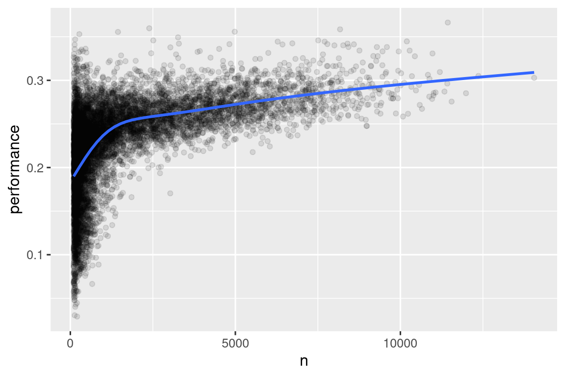
当我们绘制击球手的技能(以击球率performance衡量)与击球机会(以出局次数n衡量)时,你会看到两种模式:
-
在出局次数较少的球员中,表现的变化更大。这种情况的图形形状非常特征明显:每当你绘制平均值(或其他摘要统计量)与组大小的关系图时,你会看到随着样本量增加,变异性减小。
-
技能(performance)和击球机会(n)之间存在正相关关系,因为球队希望给他们最好的击球手最多的击球机会。
batters |>
  filter(n > 100) |>
  ggplot(aes(x = n, y = performance)) +
  geom_point(alpha = 1 / 10) +
  geom_smooth(se = FALSE)
注意将ggplot2和dplyr结合起来的便捷模式。你只需要记得从|>,用于数据集处理,切换到+,用于向图中添加层。
这对于排名也有重要的影响。如果你简单地根据desc(performance)进行排序,那么击球率最高的人显然是那些试图击球很少次数却碰巧得分的人,他们不一定是最有技能的球员。
batters |>
  arrange(desc(performance))
#> # A tibble: 20,469 × 3
#>   playerID  performance     n
#>   <chr>           <dbl> <int>
#> 1 abramge01           1     1
#> 2 alberan01           1     1
#> 3 banisje01           1     1
#> 4 bartocl01           1     1
#> 5 bassdo01            1     1
#> 6 birasst01           1     2
#> # ℹ 20,463 more rows
你可以在 http://varianceexplained.org/r/empirical_bayes_baseball/ 和 https://www.evanmiller.org/how-not-to-sort-by-average-rating.html 中找到关于这个问题以及如何解决它的很好的解释。
总结
在本章中,你学习了 dplyr 提供的用于处理数据框的工具。这些工具大致分为三类:操作行的工具(如 filter() 和 arrange())、操作列的工具(如 select() 和 mutate())以及操作分组的工具(如 group_by() 和 summarize())。在本章中,我们重点介绍了这些“整个数据框”工具,但你还没有学到如何处理单个变量。我们将在本书的“转换”部分回到这个问题,每章将为你提供处理特定类型变量的工具。
在下一章中,我们将回到工作流程,讨论代码风格的重要性,保持代码的良好组织,以便使你和其他人能够轻松阅读和理解你的代码。